toy demo

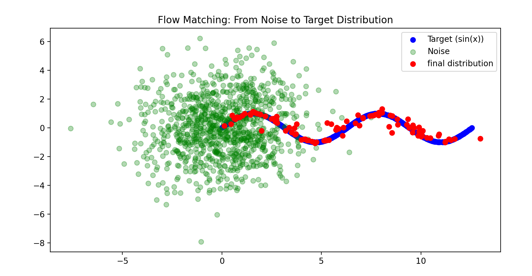
模仿这篇文章做的一个小demo,目标是在二维平面上将一堆高斯噪声中的100个点“挪”到$sinx$上。 感觉最后效果很不错啊。

import torch
import torch.nn as nn
import matplotlib.pyplot as plt
import numpy as np

# 超参数
dim = 2         # 数据维度（2D点）
num_samples = 1000
num_steps = 50  # ODE求解步数
lr = 1e-3
epochs = 100000

# 目标分布：正弦曲线上的点（x1坐标）
x1_samples = torch.rand(num_samples, 1) * 4 * torch.pi  # 0到4π
y1_samples = torch.sin(x1_samples)                      # y=sin(x)
target_data = torch.cat([x1_samples, y1_samples], dim=1)

# 噪声分布：高斯噪声（x0坐标）
noise_data = torch.randn(num_samples, dim) * 2

class VectorField(nn.Module):
    def __init__(self):
        super().__init__()
        self.net = nn.Sequential(
            nn.Linear(dim + 1, 64),  # 输入维度: x (2) + t (1) = 3
            nn.ReLU(),
            nn.Linear(64, dim)
        )
  
    def forward(self, x, t):
        # 直接拼接x和t（t的形状需为(batch_size, 1)）
        return self.net(torch.cat([x, t], dim=1))
        
model = VectorField()
optimizer = torch.optim.Adam(model.parameters(), lr=lr)

for epoch in range(epochs):
    # 随机采样噪声点和目标点
    idx = torch.randperm(num_samples)
    x0 = noise_data[idx]  # 起点：噪声
    x1 = target_data[idx] # 终点：正弦曲线

    # 时间t的形状为 (batch_size, 1)
    t = torch.rand(x0.size(0), 1)  # 例如：shape (1000, 1)
  
    # 线性插值生成中间点
    xt = (1 - t) * x0 + t * x1
  
    # 模型预测向量场（直接传入t，无需squeeze）
    vt_pred = model(xt, t)  # t的维度保持不变
  
    # 目标向量场：x1 - x0
    vt_target = x1 - x0
  
    # 损失函数
    loss = torch.mean((vt_pred - vt_target)**2)
  
    # 反向传播
    optimizer.zero_grad()
    loss.backward()
    optimizer.step()
    if epoch%1000 ==0:
        print(f"epoch:{epoch}/{epochs},loss:{loss}")

num_of_point=100
x = noise_data[0:num_of_point,:].reshape(-1,2)  # 初始噪声点
#trajectory = torch.empty(num_steps+1,2)
#trajectory[0,:]=x

tag = torch.from_numpy(np.array([1]))
# 数值求解ODE（欧拉法）
t = 0
delta_t = 1 / num_steps
with torch.no_grad():
    for i in range(num_steps):
        vt = model(x, torch.tensor([[t]], dtype=torch.float32).repeat(num_of_point,1))
        t += delta_t
        x = x + vt * delta_t  # x(t+Δt) = x(t) + v(t)Δt
        #trajectory[1+i]=x.reshape(-1,)

#print(trajectory[-1] / (torch.pi / 10 * 4))

# 绘制向量场和生成轨迹
plt.figure(figsize=(10, 5))
plt.scatter(target_data[:,0], target_data[:,1], c='blue', label='Target (sin(x))')
plt.scatter(noise_data[:,0], noise_data[:,1], c='green', alpha=0.3, label='Noise')
plt.scatter(x[:,0], x[:,1], c='red', label='final distribution')
plt.legend()
plt.title("Flow Matching: From Noise to Target Distribution")

plt.show()